The Rank function in Microsoft Excel is used to determine the position of a specific number or cell relative to a list of numbers. This function can be particularly useful when analyzing data and making informed decisions based on the relative standing of the data points.
There are several different ways to use the Rank function in Excel:
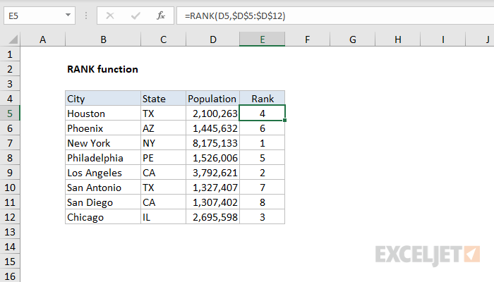
Basic Rank:
This is the most basic form of the rank function. You simply enter the formula
=RANK(number, range, [order]),
where “number” is the specific number or cell you want to rank, “range” is the list of numbers or cells you want to rank the number against, and “order” is optional and can be set to 0 for ascending order (the default) or 1 for descending order.
Rank with Equal Numbers:
If there are multiple instances of the same number in the range, the Rank function will assign the same rank to all of them.
Rank with Zero and Non-zero Numbers: The Rank function assigns a rank of 1 to the first non-zero number in the range.
Rank with Missing Numbers:
The Rank function ignores missing numbers when assigning ranks.
It’s important to note that the Rank function does not rank the cells within the range, but rather assigns a rank to each individual number within the range. Additionally, the Rank function will return an error if any of the input numbers are not unique within the range.
In conclusion, the Rank function in Microsoft Excel is a powerful tool for data analysis and decision-making. By utilizing the Rank function, you can quickly and efficiently determine the relative standing of specific numbers or cells within a list of numbers.
About Author
Discover more from SURFCLOUD TECHNOLOGY
Subscribe to get the latest posts sent to your email.