Ranking in Microsoft Excel (Spreadsheet Application)

Ranking in Microsoft Excel refers to the process of sorting data points according to their values and assigning them a rank based on that order. The RANK function in Excel is used to find the rank of a specific number in a list of numbers.

To find the rank of a number in Excel, follow these steps:

1. Ensure to select a cell where you want to display the rank.

2. In the formula bar, type “=RANK(” and then press “Ctrl + Shift + Enter”. This will insert curly braces around the formula.

3. Inside the curly braces, enter the cell reference for the number you want to find the rank of, followed by a comma and the range of cells where the numbers are.

4. Optionally, you can add a third parameter to specify the order of the values in the list. A value of 1 indicates that the RANK function should return the rank of the number in descending order, and a value of 0 indicates that the function should return the rank in ascending order.

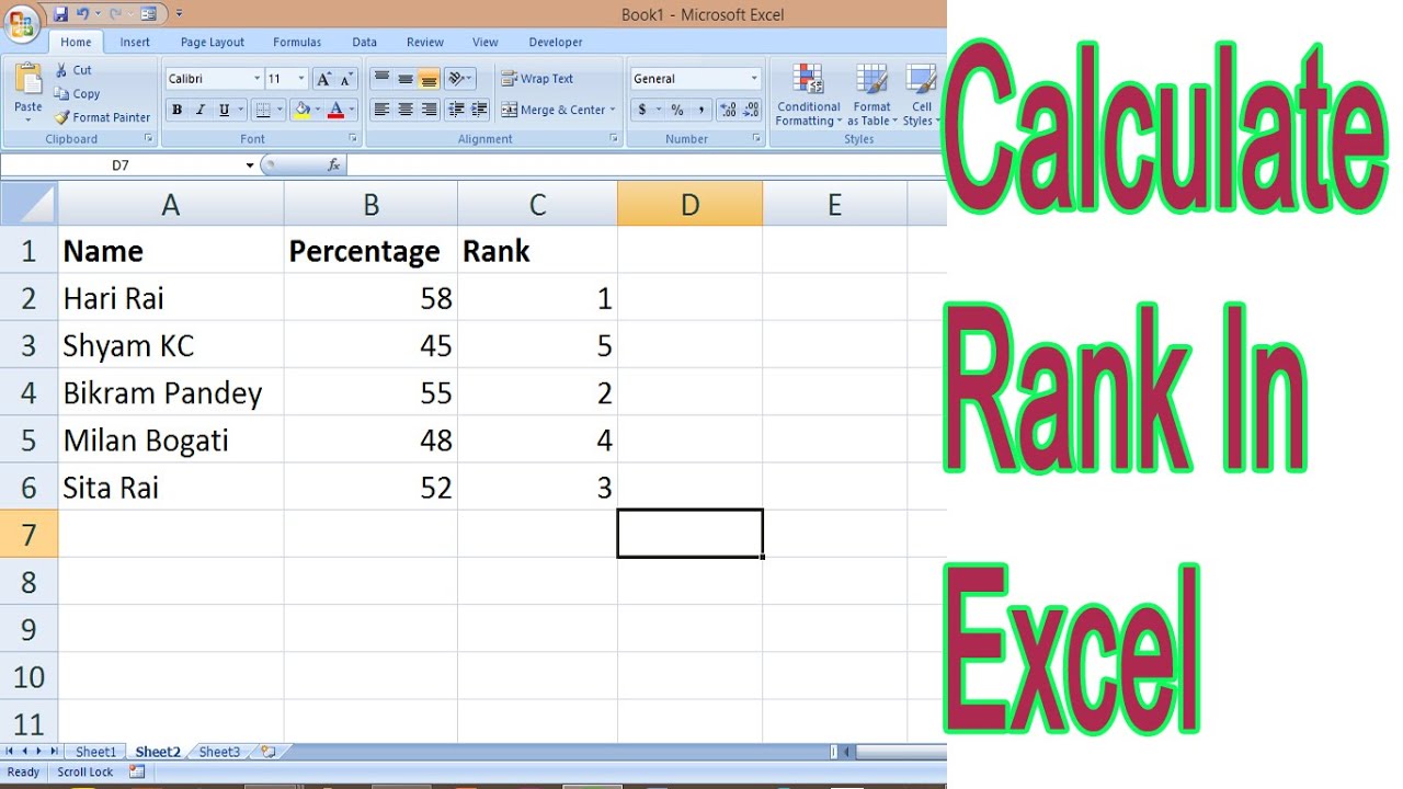
Here’s an example of how to use the RANK function in Excel:

In the  example given above, the RANK function is used to find the rank of the number in cell A1. The list of numbers is in cells A1:A5. The order of the values in the list is specified as 1, indicating that the function should return the rank of the number in descending order.

Remember to press “Ctrl + Shift + Enter” after typing the formula to create an array formula.