How to use the COUNTIF in Microsoft Excel

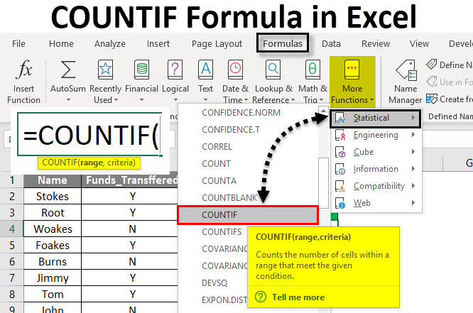
The COUNTIF function in Excel is used to count the number of cells that meet a certain criteria within a specified range.

Here’s how to use it:

1. Identify the range of cells you want to apply the criteria to. For example, A1:A10.
2. Identify the criteria you want to apply. For example, cells that contain the value “Yes”.
3. Enter the COUNTIF formula in a cell. The basic syntax is: =COUNTIF(range, criteria)
4. For the example above, the formula would be: =COUNTIF(A1:A10, “Yes”)
5. Press Enter to get the result, which in this case would be the number of cells in range A1:A10 that contain the value “Yes”.

You can also use wildcards in your criteria. For example, =COUNTIF(A1:A10, “?es”) would count the number of cells in range A1:A10 that contain any three-letter word ending in “es”.

The COUNTIFS function can be used when you want to apply multiple criteria to different ranges. The basic syntax is: =COUNTIFS(criteria_range1, criteria1, [criteria_range2, criteria2]…)

For example, =COUNTIFS(A1:A10, “Yes”, B1:B10, “>20”) would count the number of cells in range A1:A10 that contain the value “Yes” and the corresponding cells in range B1:B10 that contain a value greater than 20.