Microsoft Excel is one of the best applications that helps with performing lots of arithmetic and logical calculations in computing. However, most logical tests confuse candidates and even professionals who work at banking institutions and other financial entities.
Ensure that your column with the numerical data or grade has the right number or numerical format.
Select and click on a cell where you want or wish the letter grade to appear. For example, let’s say we have the numerical grade in cell B2, and we want the letter grade in cell C2.
Enter or feed the system with the following formula in cell C2:
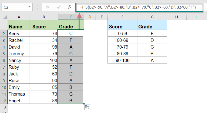
=IF(B2>=90,”A”,IF(B2>=80,”B”,IF(B2>=70,”C”,IF(B2>=60,”D”,IF(B2<60,”E”,”Error”)))))
The aforementioned function checks if the numerical grade is 90 or above, 80 or above, 70 or above, 60 or above, or less than 60. Based on the numerical grade, however, it assigns the appropriate letter grade.
If you want to use this function for the entire column, you can simply copy the formula or the function down from cell C2 to the cells below.
(Result)
Excel will automatically adjust the cell references to correspond to the correct rows.
NOTE:
Please note that this function or formula assumes a standard grading scale where grades range from 60 to 100. If your grading scale is different, you may need to adjust the formula accordingly.
About Author
Discover more from SURFCLOUD TECHNOLOGY
Subscribe to get the latest posts sent to your email.