How to Freeze Columns and Rows in Microsoft Excel

To freeze columns and rows in Microsoft Excel, you can use the “Freeze Panes” feature. This feature allows you to lock specific columns and rows so that they remain visible while you scroll through your worksheet.

Here are the steps to freeze columns and rows in Excel:

Open your Excel worksheet.

Select the column(s) and/or row(s) that you want to freeze. To select multiple columns or rows, hold down the Ctrl key while selecting.

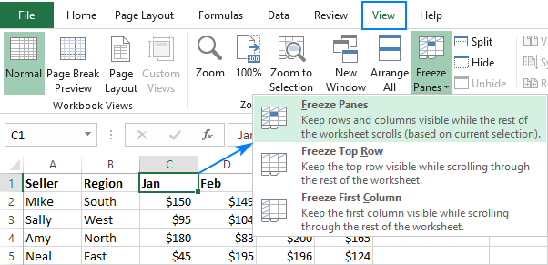
Click on the View tab

Select and click on the Freeze Panes command from the given window

From the dropdown menu, you have three options:

To freeze the selected or preferred top row, you can select and click on “Freeze Top Row”. This will keep the top row visible as you scroll.

To freeze the first column, select “Freeze First Column”. This will keep the first column visible as you scroll.

To freeze both columns and rows, you would need to select them and click on “Freeze Panes”. This will keep the selected columns and rows visible as you scroll.

Excel will apply the freezing based on your selection, and you will see a horizontal or vertical line indicating the frozen area.

You can now scroll through your worksheet, and the frozen columns and/or rows will remain visible.

To unfreeze the frozen columns and rows, you can go back to the “Freeze Panes” dropdown button in the “View” tab and select “Unfreeze Panes”. This will remove the freezing and restore the normal scrolling behavior.

About Author

SURF

See author's posts