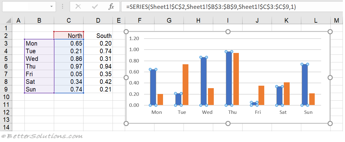
Highlight the range of cells where you want the series to appear. For example, if you want the series to start in cell A1 and end in cell A10, select the range A1:A10.
On the ‘Insert‘ tab in the Excel toolbar, click on the ‘Series’ button.
In the ‘Series’ dialog box, you can specify several options:
a. ‘Series Name‘: Enter a name for the series, if desired.
b. ‘Values’:
You can enter a constant value for each data point, such as 1 or 0. If you leave this field blank, Excel will automatically generate the series for you based on the cell range you selected.
c. ‘Formula’:
If you want to use a different mathematical formula to generate the series, you can select it from the drop-down menu. For example, if you want to create a series that doubles the value of each data point, you can select the ‘*’ formula.
d. ‘Data Labels’:
: If you want to display the data labels for each data point, you can check this box. You can also choose to display the data label on the left, right, top, or bottom of each data point.
e. ‘Line Color’:
You can select a color for the line connecting each data point.
f. ‘Line Width’:
You can choose the thickness of the line connecting each data point.
After you have specified your desired options, click on the ‘OK’ button to create the series.
Note: The series command can also be used with scatter plots, area charts, and other types of charts. Simply select the range of cells where you want the series to appear, and then follow the same steps as described above. The ‘Series’ button on the ‘Insert’ tab will then appear. Click on this button to access the ‘Series’ dialog box, where you can customize your series options.
Additionally, you can format the series after it has been created by right-clicking on the series in the chart and selecting ‘Format Data Series’. This will open the ‘Format Data Series’ dialog box, where you can make further adjustments to the appearance of your series.
About Author
Discover more from SURFCLOUD TECHNOLOGY
Subscribe to get the latest posts sent to your email.